Lightning chemistry on exoplanets and how it affects their atmospheres

Lightning leaves many traces when it occurs. In our recent paper (Ardaseva et al. 2017),  we explore which chemical traces lightning may leave in planetary atmospheres unlike our Earth. We  evaluate the chemical impact of an extreme lightning storm on planets of arbitrary composition. We predict the effect an extreme global lightning storm on the Early Earth, to see how such a storm might look like remotely.  Our model allows us to study lightning induced chemistry on exoplanets with varying chemical compositions, physical profiles and with a variety of host stars. Observers can  test our predicted values for NO, NO2 and O3 in case a balloon measurement is made in close vicinity of a lightning storm. If we were to observe an Early Earth-like extrasolar planet, we should look for nitric oxide and cyanomethylidyne (C2N) in order to identify the presence of lightning. 

Lightning is one of the most powerful events observed on our planet. The temperature inside the lightning channel is able to reach up to 30000K and pressures can increase eightfold. Such extreme conditions cause full ionization of the medium, and leave a notable impact on the composition of the atmosphere. For example, lightning on Earth is able to dissociate and ionize the very stable N2 molecule, recombining to produce 10^10 kg of NO and NO2 per year. This makes the NOx family signature molecules for lightning on the present-day Earth. But they are also signatures of human activity, since they are produced via the photodissociation of nitrous oxide, a major agricultural waste product.

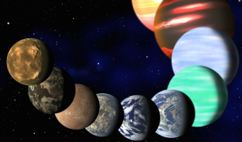
Lightning storms have been observed also on other planets in our solar system, such as Jupiter and Saturn, and are very likely to be present on exoplanets (as discussed here). The exoplanets vary in their sizes, including Earth-sized rocky planets and Jupiter-sized giants. They also vary widely in their structure and composition. Given all this diversity, how would a massive electric discharge affect their atmospheres? Does lightning affect the spectral features we could observe? Would the effect of lightning on transmission or emission spectra of exoplanets be strong enough to allow us to observationally determine the presence of the lightning storm, from chemical species that would probably not be there any other way?

Model: In order to answer these questions, we developed a model that simulates the extreme lightning storm in the atmosphere of any kind and predicts chemical impact. Our code combines 2D hydrodynamic simulation of electric discharge using ATHENA and chemical kinetic network STAND2015 with 1D atmospheric code ARGO, as described in previous work by Rimmer & Helling (2016).

Lightning storm on present-day Earth: The only example of an electric discharge event we were able to study in great detail is the lightning on Earth. In 1969, Orville et al. were able to take spectral ‘snapshots’ of discharge channel. Extreme conditions lead to the production of more complex chemicals during the cool-down. In our atmosphere, that consists mostly of oxygen (~20%) and nitrogen (~80%), a lightning event produces

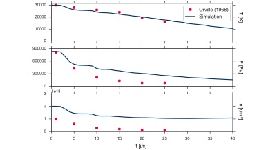
Fig 1: The temperature (T) and pressure (P) changes over time (t) during the occurrence of a lightning event.

10^10 kg of NO and NO2 per year. This makes NOx family a signature molecules of lightning on present-day Earth  We expect that signature molecules vary depending on the atmospheric composition and physical parameters of the planet.

For our model we assume that initial physical conditions (temperature, T, and pressure, p) are always the same: temperature is 30 000 K and pressure is 8 times larger (values on the very left in Fig 1). Since lightning is characterised as a bright event, we take into account radiative cooling – all the photons that are emitted and carry energy away. Therefore, the temperature, T, in Fig. one decreases with time, t.  We compare values of our model with the observations made by Orville (red dots in Fig 1). We are able to reproduce the temperature values, however the shift in pressure and number density is likely to be a result of the observational methods.

Validating by Comparing to Earth: We compared our combined model to the existing measurements of chemical mixing ratios in the Earth atmosphere. By assuming a lightning storm at 0 km altitude, our model successfully identified the signature molecules – NO, NO2.

Fig. 2: Mixing ratios from NO, NO2,O3. The red curve shows results with and the blue curves without lightning. The black dots are measurements.

Figure 2 shows the mixing ratios of NO, NO2 and O3 with (red) and without (blue) lightning. It also shows the values obtained from balloon measurements (black dots). Observers can now use our predicted values in case a balloon measurement is made in close vicinity of a lightning storm. Having reasonable agreement with all the observations, we now begin to apply our model to other more remote locations!

A case study – Early Earth: Our model allows us not only to study the present processes, but also can help to understand how the lightning storms affected the evolution of the Earth’s atmosphere as we know it now. We start our exploration with an Early Earth, when it was less than a billion years old. At this time, the composition of the atmosphere looked a bit different, with roughly 90%  nitrogen, and 10% CO2, along with trace amounts of water, hydrogen, and bon monoxide. Our model suggested, that if we were to observe an Early Earth-like extrasolar planet, we would have to look for nitric oxide and cyanomethylidyne (C2N) in order to identify the presence of lightning. The chemical output of the model can be used to predict spectral features of a planet covered with lightning storms. Our collaborators from ExoMol produced synthetic transmission spectra for both the present-day and Early Earth. Even though the signature features appear to be strong, it is not possible to resolve their features even with the upcoming JWST. We need to wait for the next generation of telescopes to find these super-powerful lightning storms!

 

A weather report for the hot Jupiter HD 189733b II.

The weather forecast of HD 189733b is further analyzed by the LEAP team, this time led by Graham Lee. They report further cloud coverage and dynamics in their newly published paper in Astronomy and Astrophysics (Lee et al. 2017).  Learn more about their results from Graham’s summary below.

In part I of this series, we coupled a radiative-hydrodynamic (RHD) atmospheric model to a microphysical cloud formation module. We simulated the atmosphere of the hot Jupiter HD 189733b and found that the planet is likely to host a highly inhomogeneous cloud structure dependent on latitude, longitude and depth of the atmosphere. In our next paper in the series, we compare our results to available Hubble Space Telescope and Spitzer Space Telescope observations of the exoplanet. We do this by post-processing our large scale cloudy RHD results using the Monte Carlo radiative-transfer (MCRT) method.

Figure 1 Images of the simulated planet at 1 micron wavelengths and at a planetary phase of 60^o (eastern terminator region). Left: Incident stellar scattered light. Right: Emitted thermal light. The cloud structures are more prominent in the left image and a twilight effect (scattering past the day-night terminator) is present. In the right image the hotter equatorial jet is very recognizable compared to the cooler higher latitude regions and the nightside of the planet. (Lee et al. 2017)

Monte Carlo radiative-transfer in a nutshell

A particular method for radiative-transfer is the Monte Carlo radiative-transfer (MCRT) technique. A MCRT simulation is a 3D stochastic, statistical sampling method of determining the local radiation field in an environment. We track the 3D random walk (or path) of millions of simulated “photon packets” through our 3D RHD simulation results. We do this by sampling a random number which govern the packets interactions with the surrounding medium. For example, if a photon packet undergoes a scattering event with a cloud particle, the new propagation direction of the photon packet is determined by sampling a random number and comparing that number to the “phase function”, which is the probability of the packet being scattered at any one angle (e.g. a random number of 0.1 could correspond to a new path slanted 10 degrees from the original direction). By simulating the path and interactions (scattering, absorption) of many millions of packets, we can count the total amount of energy escaping towards a certain direction and produce synthetic observable properties of our large scale atmospheric model. Figure 1 shows an example output from the MCRT simulations applied to our RHD model.

Figure 2  Albedo of our simulated planet compared to the observational data obtained by Evans et al. (2013). Our model is reasonably consistent with the B-band data but does not predict the drop in albedo at the V-band. Our simulation is able to decompose the effect of the different scattering material present in the atmosphere. Most scattering comes from cloud particles with a small H2 Rayleigh scattering component. (Lee et al. 2017)

Albedo/reflection spectra of HD 189733b simulation

When a transiting planet passes behind its host star, both the emitted light from the planetary atmosphere and reflected incident starlight disappear from the total luminosity of the star and planet system, resulting in a dip in observed flux of the system during the secondary eclipse of the transit. The albedo of a planet is defined as the fraction of incident starlight that is scattered back into space. For example, a planet with an albedo of 0.2 at a wavelength of 300 nm, returns 20 % of the incident star light at 300 nm back into space. The albedos of many hot Jupiter planets have been measured by the Kepler space telescope, and some by the Hubble Space Telescope. Figure 2 shows the albedo of our HD 189733b simulation produced from the MCRT simulation compared to the geometric albedo observations using the Hubble Space Telescope by Evans et al. (2013). We also combine our albedo and emission spectra to compare to dayside observations of HD 18973b from Hubble and Spitzer Space Telescopes (Fig. 3).

Figure 3  Dayside luminosity ratio of our simulated planet compared to HST and Spitzer measurements (Evans et al. 2013, Crouzet et al. 2014, Barstow et al. 2014 and Knutson et al. 2012). Our simulation compares well to the observed trends in the dayside emission spectra. (Lee et al. 2017)

We find that our model is generally consistent with the observations but has some offsets with some data points. However, we do not fit the “V-band” (Visible wavelength range) dip in albedo as observed by the HST measurement. This suggests the presence of an absorbing material present in the atmosphere of HD 189733b which was not accounted for in our modelling. This absorber has been noticed in other hot Jupiter planets and it is currently a mystery what causes these dips in albedo at these wavelengths. Overall though, this general agreement with the observations suggests that the cloud coverage and temperature structures of our large scale simulation are probably a reasonable expectation of the dayside properties of HD 189733b.

Figure 4  TESS and CHEOPS predicted dayside albedos and bandpasses (dashed line). CHEOPS has a larger albedo due to the effect of photons scattered by clouds at optical wavelengths, which TESS is not sensitive too. (Lee et al. 2017)

Predictions for TESS and CHEOPS

We also produce predictions of the geometric albedo and phase curve behaviour of HD 189733b for the upcoming NASA Transiting Exoplanet Space Survey (TESS) and ESA CHaracterising ExOPlanets Satellite (CHEOPS). Figure 4. shows our results shows our TESS and CHEOPS predictions, and includes a Kepler prediction (even though HD 189733b will not be observed by Kepler) for comparisons. We found that our simulated dayside atmosphere would be 10% brighter when viewed by the CHEOPS mission compared to the TESS instruments. This is due to the fact that CHEOPS is more sensitive to the optical scattering component (cloud cover), as TESS is more sensitive to infra-red thermal emission from the planet. By comparing the albedos and phase curves between the CHEOPS and TESS instruments, an idea of the extent of the cloud coverage on the observed planet may be inferred. This may be useful for helping decide which planets to observe with more time limited spectroscopic instruments such as the James Webb Space Telescope (JWST).

Figure 5  RGB channel GIF of the incident scattered light varying with planetary phase. The real planet is probably slightly bluer than the brownish colour presented here due to an unknown absorber at visible wavelengths (See Fig. 2; Lee et al. 2017).

RGB channel phase curves

Lastly, we produced a RGB channel phase curve output using the albedo results. This is provided in GIF form in Fig. 5. The real planet is likely to be slightly bluer than the reddish brown colour presented due to the unknown V-band reducing the R channel’s magnitudes.

For more details check out the original paper on ADS:

G. Lee, K. Wood, I. Dobbs-Dixon, A. Rice, Ch. Helling, 2017, A&A, 601, A22

The LEAP Group can be found here:

http://leap2010.wp.st-andrews.ac.uk/

And finally, don’t forget to like us on Facebook:

https://www.facebook.com/leap2010

A weather report for the hot Jupiter HD 189733b I.

One of the most prominent and visual features of weather phenomena on Earth are water clouds which govern a large part of Earth’s climate. In Lee et al. (2016), the first of a series of papers, we investigated what the atmosphere of the hot Jupiter exoplanet HD 189733b may look like, in particular what the properties of clouds that maybe present in the atmosphere are. We used a computer simulation of the atmosphere of the hot Jupiter exoplanet HD 189733b including, for the first time, a microphysical description of 3D cloud particle behaviour in the atmosphere.

Simulating a cloudy exoplanet atmosphere.

A major tool for the exploration of the properties of Earth, Solar System and Exoplanet atmospheres are the use of Radiative-Hydrodynamic (RHD) or Global Circulation Models (GCM). These models simulate the temperature, pressure and other important properties of an atmosphere by evolving the equations of geophysical fluid dynamics, representing the large scale motions or “winds” of the atmosphere. The motions of the atmosphere depend on numerous factors such as the rotation rate, which affects the fluid flows primarily through the Coriolis force; pressure gradients, causing flows of gas. These models also take into account the heating from an external source onto the atmosphere, primarily radiation from the host star of the exoplanet. For hot Jupiter atmospheres, the intense effect of heating on dayside of the planet has large consequences on the specific weather properties, driven primarily from the large temperature differences between dayside and nightside regions of the planet.

Figure 1. The number density of cloud particles at 1 mbar pressure in the HD 189733b simulation. A build up of material at the equator near 270 degrees longitude is seen. Arrows show the direction and strength of the atmospheric flow. The dynamics is dominated by the strong super sonic equatorial jet which efficiently transports cloud particles around the globe (Lee et al. 2016).

In our study we used the RHD model from Dobbs-Dixon & Agol (2013) of the hot Jupiter HD 189733b and coupled it to our microphysical based cloud formation model, the details of which can be found in our numerous other blog posts (here and here). We found that our simulated cloud structures varied significantly in latitude, longitude and depth of the atmosphere. Cloud particles were more numerous of the nightside of the planet compared to the dayside regions, primarily due to the fast winds flowing from the dayside to the nightside slowing down as they approached the western terminator region. This creates a “traffic jam” effect, where cloud particles pile up on the western terminator nightside (Fig. 1).

Figure 2. The average cloud particle size in micron at 10 mbar pressure in the HD 189733b simulation. A large difference in cloud particle sizes between dayside and nightside as well as latitude is apparent (Lee et al. 2016).

Cloud particle sizes were also very different from the dayside to the nightside. On the dayside, the hotter temperatures evaporate the more volatile Magnesium containing materials MgSiO₃ and Mg₂SiO₄, while these materials are stable on the nightside of the planet. This leads to different particles sizes, smaller particles of ~nm sizes on much of the dayside and ~μm sized particles on the nightside (Fig. 2).

Latitudinal differences in cloud particle size are also seen, with the hot equatorial super-sonic jet containing no Mg containing materials, and only the very stable TiO₂ and SiO₂ minerals. Higher latitudes, where it is cooler, contained ~90%+ Mg bearing materials. In our simulations we see bands of different materials dependent on the atmospheric properties, similar to how the bands of different materials on Jupiter colour different bands.

Figure 3. A collage of atmospheric properties at the equator of the simulated planet. The radial numbers denote the atmospheric pressure in log_10 bar. Numbers on the outside of the ring denote longitude. Top row: Gas temperature, cloud particle number density, cloud particle mean radius. Middle: TiO2 abundance, SiO abundance, SiO2 abundance. Bottom: MgSiO3 abundance, Mg2SiO4 abundance. Clear differences in the cloud properties can be seen in longitude and depth. For example, the dayside of the planet contains a large region of TiO2, while the nightside has more silicate materials present (Lee et al. 2016).

Overall, our results show that we can expect very cloudy, dynamic weather on HD 189733b, with cloud particles evaporating and condensing constantly as they are pushed along with the winds from dayside to nightside. However, unlike the temperate conditions on Earth, these cloud particles would be travelling at super-sonic speeds, dwarfing by magnitudes the most violent hail storms found on Earth.

In part II of our weather report, we will look at simulating the observable properties of our RHD modelling results and comparing our modelling efforts to Hubble Space Telescope and Spitzer Space Telescope data of HD 189733b.

For more details check out the original paper on ADS:

G. Lee, I. Dobbs-Dixon, Ch. Helling, K. Bognar, P. Woitke, 2016, A&A, 594, A48

The LEAP Group can be found here:

http://leap2010.wp.st-andrews.ac.uk/

And finally, don’t forget to like us on Facebook:

https://www.facebook.com/leap2010

Carbon planets and diamond clouds

Could diamond planets exist? Probably not, but what about carbon-planets in more general terms? So far, almost all discovered planets were oxygen-rich. The quest about carbon-rich planets touches fundamental question of astrophysics, including how stars formed in the early universe and how planets form in disks around young stars. Ultimately and somewhat surprisingly perhaps, we are required to understand what kind of clouds form in atmospheres of carbon-rich planets in order to disentangle existing observations or to predict possible observations, because clouds do act like an optical and a thermal blanket to the planet below it. Therefore, Helling, Tootill, Woitke & Lee (2016) set out to model cloud formation in carbon-rich atmospheres. They find that the material composition and, hence, the appearance of carbon-rich planets (possibly WASP-12b or HR 8799 b, c, d, e) drastically differs from the well-studied oxygen-rich giant gas planets (like HD 189733b or HD 209458b). They show, that only the very inner parts of a carbon-cloud could possibly be made of diamond crystals, making it a rather darkish type of planet.

Stars come with all sorts of chemical ‘tastes’: Those with more oxygen than carbon (called ‘oxygen-rich’), and those with more carbon than oxygen (called ‘carbon-rich’). Stars in the present universe are born as oxygen-rich and only change to carbon-rich at later stages in their life-time when they become giant stars with diameters of hundreds of stellar radii. Therefore, extrasolar planets are expected to be oxygen-rich.

Observations start to indicate that some extrasolar planets maybe carbon-rich, or at least have enough carbon-molecules in their atmospheres so that our telescopes can see them. For example, WASP-12b was suggested to be carbon- rich (Madhusudhan et al. 2011) but a second observation could not confirm that finding (Kreidberg et al. 2015). Four planets of the planetary system HR 8799 have tentative detections of C₂H₂, CH₄, and CO₂, all rather large carbon-binding molecules (Opennheimer et al. 2013).

Planets only form in disks around young stars and young stars are oxygen-rich. Stars only turn carbon-rich at later ages. So, why should carbon-rich planets exist at all?

Figure 1: The top panels show the material composition that we predict from our cloud models in per cent: 1.0 means that the cloud particles are made to 100% of this material (e.g. Al2O3 – light blue, carbon – grey) and 0.2 means that the cloud particles contain 20% of that material (e.g. Mg2SiO4 or MgSiO3 – yellow/orange). Different lines represent different materials. The lower pictures visualize how the cloud would look like if we were able to observe it more closely: An oxygen-rich giant planet (left) would sparkle in different colours while a carbon-rich planet would look rather dull and dark-grey (Helling et al. 2016).

Here are three ideas how this could work:

1) Extremely carbon-rich stars formed in very early universe (Mashian & Loeb 2016). These carbon-rich stars were young at some point and may therefore have formed carbon-rich planets. The problem with that hypothesis is that our Sun is oxygen-rich and not that old. The Sun is a young star compared to the stars we know of in our present universe. It is therefore highly unlikely that any presently observable carbon-rich planet has formed in the early universe.

2) Carbon-rich stars in our present-day universe bath their originally oxygen- rich planets in a strong wind that carries large amounts of carbon-rich gas and dust. As this wind continues to hit the planets atmosphere, it increases slowly but steady its carbon content and appear as carbon-rich at some point. The obvious conclusion is that all carbon-rich stars with strong mass losses should have carbon-rich planets. This has not been observed so far.

What are we left with? We need to take a closer look at the star and planet formation processes and see whether chemical niches appear that allow us to explain the possible emergence of carbon-rich planets or episodes of carbon- enrichment. In other words, we need to study how the local chemistry changes in planet-forming disks that emerge around young stars in order to conserve the angular momentum of the collapsing gas-cloud that will form a young star. This local chemistry will play a large role in determining what kind of planets will form in such disks. Hence, the beauty lies in the detail.

Knowing about the problem, we have merged our expertise in atmosphere modelling (Christiane Helling) and planet-forming disk modelling (Peter Woitke). Through this work, published in the Life journal in 2014, we realized that we need to understand cloud formation a lot better in order to be able to say if the chemical composition of a planetary atmosphere would be carbon-rich or oxygen-rich.

In Helling, Tootill, Woitke & Lee 2016 we worked out a model that would allow us to predict how clouds form in carbon- rich atmospheres. The oxygen-rich case was well studied already and we could build on our experiences with it.

Figure 1 visualises our main results. The left-hand panel shows the results for the cloud layer that forms in an oxygen-rich atmosphere of a planet, the right-hand side shows the cloud forming in the carbon-rich planet. Here are the three main observations from Figure 1:

a) Clouds in oxygen-rich atmospheres are made of 40% silicates like Mg₂SiO₄ and MgSiO₃, 20% SiO, 10% iron, with the remaining 30% being a mix of other materials.

b) Clouds in carbon-rich planets would be made of a minimum of 60% carbon with the remaining 40% (or less!) being a mix of other carbon-binding materials and iron.

c) While silicate clouds in oxygen-rich atmospheres are semi-transparent at the top and dark further inside, carbon-clouds are graphite-black at the top and diamond-clear further inside.

It appears that an oxygen-rich planet with strong winds should be much more beautiful to observe because many mineral cloud particles could appear in many colours. Carbon-rich planets would look rather dull and grey in comparison.

For more details check out the original paper on ADS:

Helling, Tootill, Woitke & Lee 2016, eprint arXiv:1612.01863

The LEAP Group can be found here:

http://leap2010.wp.st-andrews.ac.uk/

And finally, don’t forget to like us on Facebook:

https://www.facebook.com/leap2010

EXO-LIGHTNING Part II: a planet and its radio signal

How big a lightning storm would we need to produce an observable signal on an exoplanet? What effect would such a storm have on the local atmosphere of the planet? These questions are explored in the paper by Gabriella Hodosán, Paul B. Rimmer and Christiane Helling for the mini-Neptune HAT-P-11b discovered by the Hungarian-made Automated Telescope Network (HATNet) in 2009.

 

Artist’s impression of an exoplanet like HAT-P-11 (Credit: NASA/JPL-Caltech).

HAT-P-11b is a Neptune-like exoplanet, orbiting the host star at a distance of 20 times shorter than the Earth-Sun distance. It is about 5 times bigger in size than Earth and 26 times more massive. It was discovered by the transit technique. In 2009 a group of scientists (Lecavelier des Etangs et al. 2013) observed the planet at a radio frequency band centred at 150 MHz. The observation was timed so that the planet would be observed before, during and after its occultation. They found a radio signal of ~4 milliJansky (mJy), which vanished as the planet passed behind its host star. The French team suggested that this signal could come from the planet, as it disappeared when the planet was behind the star. In 2010 they had a re-observed the planet, but could not find the signal this time. If the radio signal in 2009 was real, than its absence in 2010 suggests that it was produced by a transient event.

A storm with millions of lightning flashes

In our work (Hodosán, Rimmer and Helling 2016) we assumed that the signal detected in 2009 was real and was coming from the planet, as was suggested by the original paper. The question that raised our curiosity was: Could such a radio signal be produced by lightning in the planet’s atmosphere, and if yes, how many lightning flashes would be needed for it? In order to answer this question, we assumed that the basic lightning physics is the same on Earth, on the Solar System planets and on exoplanets. We previously used this assumption in Bailey et al. 2014 (see the blog entry here). Based on these assumptions we calculated that ~4×10⁶ lightning flashes over a km² in an hour should have happened during the observations of HAT-P-11b, over its whole disk.

Artist’s concept of lightning on Venus (Credit: ESA/image by Christophe Carreau)

Is this enormous number of lightning flashes unreasonable? Our group (e.g. Lee et al. 2015, Helling et al. 2016) and others (e.g. Heng & Showman 2015) have shown that exoplanets orbiting really close to their host star have very dynamic atmospheres, meaning that they change continuously, producing clouds of different sizes all over the planet’s surface (e.g. our posts here and here). HAT-P-11b, being so close to the star, is likely to have a hugely dynamic atmosphere, which could allow the formation of immense thunderclouds, similar to the big red spot on Jupiter, focusing the lightning activity to a certain regime of the planetary surface, such as the face of the planet, which was observed in 2009.

Flash densities and optical emission of lightning that would produced the observed radio signal (Hodosán et al. 2016)

Visible in the optical range?

Could we see such a huge storm with optical telescopes, in the visible range of the spectrum? Because a very large number of lightning flashes would be needed to produce the observed radio signal, they would produce a very high optical emission. We found that, depending on the energy emitted by the lightning flashes, the optical emission of this enormous thunderstorm would be comparable to that of the host star HAT-P-11, a bright K star, or would even outshine it. This is quite unlikely to happen, so we concluded that the radio signal was most probably not a result of lightning storms of HAT-P-11b.

Could we trace chemical signals of such a storm?

However, we were curious to find out how the local chemistry would change because of he large amount of lightning happening at a time. It is known from Earth that lightning has an effect on the chemistry of the atmosphere where it occurs. The process of discharging a lightning channel involves very high temperatures and the release of a large amount of energy. This results in chemical reactions that would not occur any other way. So-called „non-equilibrium” species are produced. These only stay in the atmosphere for a relatively short amount of time, then they turn into their equilibrium counterparts, unless the conditions became appropriate for their production. For example lightning on Earth produces NO₂ in the atmosphere, which disappears after a while, unless more lightning occurs and produces more of this molecule.

In our study, we found that HCN would be the species to look for in the case of HAT-P-11b, if we want to observe lightning. Interestingly, we would not need the obtained number of lightning flashes to produce observable signatures, but orders of magnitude lower lightning activity would still be capable of creating observable quantities of HCN. These signatures would appear in the infrared band for 2-3 years after the occurrence of the storm, if lightning would have happened at a certain height of the atmosphere.

Lightning or aliens?

Since the press release (now showing previous, out-dated results) of the paper, several newsagents picked up the story. Some of them focused on our interpretation of an “unexplained radio signal” with a natural phenomenon (i.e. lightning) instead of aliens. This gave us the idea of comparing our study with previous ones looking for alien radio signals coming from space.

“Two possibilities exist: either we are alone in the Universe or we are not. Both are equally terrifying.” – Arthur C. Clarke

Allan Telescope Array (Credit: SETI Institute).

The question whether Earth is the only place in the Universe that hosts life on its surface has been around, unanswered, for thousands of years. We can go even further: are there other civilizations, intelligent races, out there? One of the first scientific papers on the question was written by G. Cocconi and P. Morrison, who wrote down the theory of ways of interstellar communication. Frank Drake started the so called “Project Ozma”, the first systematic search for alien signals with a radio telescope. His attempt was well designed, however, unsuccessful, such as all attempts have been so far. A year later, he organized a conference. While he was preparing for it, he came up with the idea of the famous Drake equation, which relates the number of intelligent civilization in our Galaxy to a series of factors. Since then several papers have been published about different theories of what the signatures could be of such intelligent civilizations, could we detect any of those signatures and why haven’t we detected any signs of them.

When looking for extraterrestrial intelligent life, we have to consider the signature most promising to look for. Radio waves propagate through space almost unimpeded and with the speed of light, making these wavelengths of the electromagnetic spectrum good candidates for ET signs. However, the electromagnetic spectrum contains a wide range of radio frequencies. Then where to look? The frequency band called “microwave window” is the favoured part of the spectrum, ranging from 1 GHz to 10 GHz. Physically this is the most quiet range of radio frequencies, meaning that this part is the less contaminated by natural radio emission. However, it is not free of it. But then how can we distinguish between a natural and non-natural radio emission? In theory, a radio signal produced by some kind of technology would be narrow-band. It would emit only in a very narrow range of frequencies. While natural phenomena would have broadband emission, emitting with a gradually increasing/decreasing power through out a wide range of frequencies.

Now, what about radio emission coming from lightning? Two main aspects of the technology-emitted radio signal and the lightning-caused radio signal are very different. Lightning emits in a broad spectral band, such as most of the natural phenomena we know of. The second main difference is the frequency at which it emits. While we expect other extraterrestrial civilizations to broadcast their signals at the GHz range, lightning emits mostly in the kHz up to a few hundred MHz frequency range. The radio signal from HAT-P-11b was observed in radio band centred at 150 MHz. This is much lower than what we would expect from an ET broadcast. However, this is the higher part of the radio band where lightning could still emit.

So in summary, the radio signal from HAT-P-11b is most probably not an alien signal, but either caused by a natural phenomenon, or simply instrumental noise. If we were the ones broadcasting radio signals towards other planets, we would not do it from a definitely uninhabitable planet, like the hot, Neptune-like HAT-P-11b. We would also not broadcast at frequencies, which would be difficult to observe due to natural noises, like at 150 MHz.

So the conclusion?

Credit: ESA

The conclusion is that there are various explanations, all from natural phenomena, which could cause a weak radio signal like the one observed by Lecavelier des Etangs et al. (2013) in 2009. However, most probably it is not lightning. We have to emphasize though, that lightning might be very different on an exoplanet from what we know in the Solar System. Exo-lightning may be much more energetic, producing more powerful signatures than has ever been observed in our Solar System. In which case, lower number of flashes, within the reasonable range, could produce observable signatures.

However, the importance of our study is that it showed that in the future, combined radio and infrared observations may lead to the first detection of lightning on an extrasolar planet, though this planet will most probably be closer to us than HAT-P-11b is. It also shows an original scenario for the explanation of radio emission observable on planets outside our Solar System.

If you have an opinion, please leave a comment below.

For more details check out the original paper on ADS:

 Hodosán, G.; Rimmer, P. B. and Helling, Ch, MNRAS, 461, 1222, 2016

The LEAP Group can be found here:

http://leap2010.wp.st-andrews.ac.uk/

And finally, don’t forget to like us on Facebook:

https://www.facebook.com/leap2010

EXO-LIGHTNING Part I: what can we learn from the Solar System?

Is lightning a phenomenon only occurring on Earth? Or is it universal? How can the knowledge we learnt from Solar System lightning help with discovering lightning on exoplanets and to understand these very different worlds? The next two entries will be devoted to the work on extraterrestrial lightning carried out by Gabriella Hodosán, LEAP PhD student, under the supervision of LEAP PI Dr Christiane Helling, in collaboration with various LEAP group members. In Part I we apply results of lightning surveys of several Solar System planets, including Earth, to different groups of extrasolar planets. Part II will be about a specific planet, HAT-P-11b and the possibility of lightning detection in its atmosphere.

Lightning is one of the most spectacular phenomena on Earth. It has interested not just scientists but the general public for thousands of years. However, it is not a unique phenomenon to Earth. It has been observed before on several Solar System planets, such as Jupiter, Saturn, or Uranus and Neptune. Spacecraft like Cassini, Galileo, New Horizons or the Voyagers provided us with breath-taking images of the outer Solar System, including images and measurements of lightning occurring on the gas giant planets (Fig. 1).

Figure 1. Lightning on Jupiter (right top and bottom) and Saturn (left bottom). (Credit: NASA/JPL-Caltech/SSI, NASA/Galileo)

Since the late 90s, thousands of exoplanets have been discovered. These exoplanets show a large diversity (Fig. 2) in sizes, masses, even distances to the host star, much different to our Solar System planets: Jupiter-size planets orbiting other stars at the distance of Mercury; planetary systems with several planets inside the orbit of Mercury; terrestrial planets several times bigger than Earth, but still rocky and not made of gas. Could these planets host lightning in their atmospheres? Let’s look at Earth and Saturn. They have different composition, different sizes, masses, different atmospheres. And still, they both show lightning activity. So why couldn’t it occur on exoplanets?

Figure 2. Diversity of exoplanets and brown dwarfs on a mass-radius and distance-density plot. The lines on the top plot indicate the potential chemical composition of the bodies based on their obtained mass and radius  (Hodosán et al. 2016).

In our work, we were focusing on the statistical side of lightning occurrence on Solar System planets, then extrapolated to extrasolar objects. Lightning climatology explores the spacial and temporal distribution of lightning. It uses the quantity of flash rate [flashes/unit time, e.g. flashes/hour] or flash density [flashes/unit time/unit surface area, e.g. flashes/hour/km²] to quantify this distribution. It is a tool to estimate the lightning activity on the surface of an object. This is important in order to estimate the total energy released of lightning flashes, and to determine whether the signatures produced by lightning would be observable from Earth.

Earth

Lightning observing networks net the whole surface of the Earth and satellites continuously look for lightning flashes from near Earth orbits. Lightning monitoring is important because of the hazards (e.g. forest fires, large scale power outage, fatalities) it causes. Measurements from Earth provide the largest data sets we can work with. In our study we analyzed data from the Lightning Imaging Sensor (LIS)/Optical Transient Detector (OTD), which are optical instruments on board of satellites, and from two ground based radio networks, the Sferics Timing and Ranging Network (STARNET) and World Wide Lightning Location Network (WWLLN). Figure 3 shows an example of lightning climatology maps produced from LIS/OTD data. It shows an average of lightning occurrence over the period of 1995-2013. It shows clear trends of more lightning over continents than over oceans, and more lightning over lower latitude regions than higher latitude regions.

Figure 3. LIS/OTD lightning climatology map averaged from 1995-2013 (Hodosán et al. 2016).

Lightning occurs not only in thunderclouds but in volcano plumes as well (e.g. see work by our group, and the eruption of Eyjafjallajökull). Based on literature research we collected flash densities from two volcano eruptions: Mt Redoubt in 2009 and Eyjafjallajökull in 2010. Some interesting fact: both eruptions show orders of magnitude larger flash densities than what thunderclouds produce. On average the LIS/OTD data showed a 2×10^-4 flashes/km²/h flash density while Eyjafjallajökull showed 0.1 – 0.32 flashes/km²/h and Mt Redoubt produced up to 2000 flashes in an hour over a square kilometer.

Venus, Jupiter and Saturn

Is there lightning on Venus? The long debated question has not yet been fully answered, however, more and more clue indicate the existence of such phenomenon on Earth’s sister planet. If lightning does exist on Venus, it is probably not very energetic and it appears deep within the atmosphere, since no optical observation of it has been made to date. Radio data from the Venus Express mission, however, shows a possible ~10^-11 flashes/km²/hour flash density.

Figure 4. Lightning distribution on Jupiter. Triangles: Galileo data from 1997. Circles: New Horizons data from 2007.

Jupiter and Saturn are more interesting, since, apart from Earth, these are the only planets in the Solar System where lightning has been observed directly. We used published data from the Galileo (1997, Jupiter), New Horizons (2007, Jupiter) and Cassini (2009, 2011, Saturn, e.g.) spacecraft. Figure 4 shows and example lightning distribution map for Jupiter. It shows and increased lightning activity around the +- 50-degree latitude regions, most probably due to the increased affect of internal heating on convection and cloud formation. Until 2009, only radio signals of lightning were observed on Saturn. The so-called SEDs (Saturnian Electrostatic Discharges) are short and strong radio bursts from lightning, detected by e.g. the Voyagers and Cassini spacecraft. The two giant gas planet, on average, shows a flash density of 10^-6 – 10^-7 flashes/km²/hour.

Exoplanets

Now the most exciting part: How does this all relate to exoplanetary research? The idea behind our paper is to use the statistics from Solar System planets to estimate a possible lightning occurrence on exoplanets with similar environments to those described in the previous sections. E.g. let’s take possible ocean planet: Kepler-62f. Then apply the flash density derived for Earth for above oceans: ~5 x 10^-5/km²/hour. Combining this, we estimate the flash density on Kepler-62f, throughout its whole surface, to be the same: ~5 x 10^-5/km²/hour. Another example is to apply the flash densities in order to estimate the total lightning occurrence during the transit of a planet. 55 Cancri e is a close-in rocky planet, most probably cover by lava. How much lightning could occur during its transit on the projected disk of the planet, if we assume continuous flashing from volcano activity? Depending on which eruptions we consider as the template, 55 Cnc e could produce as many as 10⁸-10¹² flashes on its whole disk during its 1.5-hour transit. This enormous amount of lightning would produce radio emission that might be observable during the transit.

In Part II we introduce our original idea of estimating whether a weak and tentative radio signal observed on the mini-Neptune, HAT-P-11b, could have been caused by lightning or not.

If you have an opinion, please leave a comment below.

For more details check out the original paper on ADS:

 Hodosán, G.; Helling, Ch; Asensio-Torres, R.; Vorgul, I.; Rimmer, P. B., MNRAS, 461, 3927, 2016

The LEAP Group can be found here:

http://leap2010.wp.st-andrews.ac.uk/

And finally, don’t forget to like us on Facebook:

https://www.facebook.com/leap2010

The mineral clouds on the extrasolar giant gas planets HD 209458b and HD 189733b

The giant gas planets HD 189733b and HD 209458b are the two most studied extrasolar planets today. Both have been observed by several research groups with varies telescopes including the Hubble and the Spitzer Space Telescopes, and the super-high-precision HARPS spectrograph mounted on the 3.6 m telescope in La Silla in Chile. These extensive observational programs have reviled details about the atmospheres of these planets, like for example the presence of CO and CH₄ in HD 189733b and CO and H₂O in HD 209458b. Observations have further established that both gas giants form clouds inside their atmospheres (e.g. Sing et al. 2016). Are these clouds similar to clouds on Earth? What are they made of? Why does HD 209458b seem to have more water vapour than HD 189733b? How different are clouds between the two planets?

We use results from 3D radiative-hydrodynamics simulations of the atmospheres of HD 189733b and HD 209458b to answer the above questions and to derive cloud characteristics. We apply the same ideas about cloud formation as described in our Drift-Phoenix post. First, condensation seeds form with a certain efficiency. Once they are present, many solid materials (e.g. MgSiO₃[s], Fe[s], SiO[s], TiO₂[s], [s] meaning solid phase) can condense on these numerous but small surfaces. As these cloud particles grow, they fall into the atmosphere (gravitational settling). These raining cloud particles will encounter changing ambient conditions because the gas temperature and the gas pressure increase inwards the atmosphere. On their way, the cloud particles change in size but also in composition.

We now probe the atmospheric cloud formation in HD 189733b and HD 209458b by calculating the cloud structure for the vertical atmosphere at different longitudes and latitudes shown on Fig. 1.

Figure 1. Points in the atmosphere where cloud formation was probed

We find that both planets have the smallest cloud particles near the top of the cloud and the largest cloud particles at the bottom of the cloud, which is far inside the atmosphere beyond observable heights. This can be seen from the black solid line in all the panels in Fig 2.

Figure 2 demonstrates the vertical cloud structures for the daysides of the giant gas planets HD 189733b (top) and HD 209458b (bottom). We show how the material composition changes with height for different latitudes (Φ=270°, 315°, 0°, 45°, 90°) along the equator. The material composition is visualized by the lines of different colours, representing one material each: TiO₂[s] – solid dark blue, Al₂O₃[s] – solid blue, CaTiO₂[s] – solid purple, Fe₂O₃[s] – dashed light green, Fe[s] – dotted green, SiO[s] – dashed brown, SiO₂[s] – solid brown, MgO[s] – dashed dirty orange, MgSiO₃[s] – dashed orange, Mg₂SiO₄[s] – solid orange. The contribution of the different materials to the volume of the cloud particles, V_s/V_tot, is shown in percentage. For example, V_Mg2SiO4/V_tot=0.3 means 30% of the cloud particle is made of Mg₂SiO₄.

Figure 2. Dayside cloud particle material composition (colour coded, left axis) and mean grain sizes (black, right axis) for both exoplanets. For colour codes refer to the original paper at Helling et al. 2016, fig. 7, or to the text above

To the left in Fig. 2, where the gas pressure is low, is the upper part of the atmosphere and the cloud. Here, the cloud particles are small (10^-2 μm) and made of a rich mix of materials indicated by many coloured lines appearing in the plots of Fig 2. Letting your eyes wonder more to the right shows that most of the lines disappear, because these materials evaporate (like Fe₂O₃[s], MgO[s]). Most of the cloud particles are now made of MgSiO₃[s], Mg₂SiO₄[s], SiO₂[s] and a bit of Fe[s]. When moving further inwards the atmosphere where the temperature increases beyond thermal stability of the silicate materials, a larger fraction of cloud particles will be made of Fe[s].

Inspecting Fig 2 a bit closer by comparing the results for HD 189733b and HD 209458b shows that the cloud particles at the inner rim of HD 189733b are more Fe[s] rich than for HD 209458b. The cloud particles in the upper atmospheric regions appear rather similar in material composition: they are made of silicates and oxides with only very small contribution form iron.

A major result of our work is that all cloud properties are interlinked and that it is extremely difficult to guess correct combinations of cloud particle-sizes and their material composition that will occur at a certain place inside the atmosphere of an extrasolar planet.

Why would HD 209458b show more water absorption than HD 189733b? Hence, why does HD 209458b seem to have more water vapour than HD 189733b according to observations? Water is the most abundant absorbing species in the gas phase and maybe one would not expect any differences between two relatively similar planets like HD 189733b and HD 209458b. However, our research shows that a considerably larger portion of the atmosphere of HD 209458b is affected by the cloud than for HD 189733b. The clouds in HD 209458b reach into regions of lower atmospheric pressure, hence lower gas densities, compared to HD 189733b. It should therefore be more difficult to observe water on HD 209458b than on HD 189733b. Therefore, the more a cloud layer extends into the low-density upper part of the atmosphere, the shallower the gas-absorption features will be in the observed spectrum (Fig. 3).

Figure 3. More water molecules accumulate above clouds at higher atmospheric pressure. Clouds on HD 209458b form lower in the atmosphere (right), therefore have more water molecules above them resulting in a deeper water absorption feature in the spectrum, than on HD 189733b (left)

 

For more details check out the original paper on ADS:

 Ch. Helling, G. Lee, I. Dobbs-Dixon, et al. 2016, MNRAS, 460, 855

The LEAP Group can be found here:

http://leap2010.wp.st-andrews.ac.uk/

And finally, don’t forget to like us on Facebook:

https://www.facebook.com/leap2010

Interdisciplinary thinking: Atmospheric electrification in the Solar System and beyond

According to Wikipedia, interdisciplinarity involves the contribution of two or more academic disciplines to allow progress through recognition of different ways of thinking. Driven by curiosity, a group of researchers from the disciplines of plasma physics, meteorology, volcanology and astrophysics (observations and modelling of brown dwarfs, exoplanets, protoplanetary disks) met in the Scottish Highlands in Pitlochry in 2014 to discuss their research on ‘Electrification in dusty atmospheres inside and outside the solar system’. This workshop was the inspiration for a review articles ‘Atmospheric electrification in dusty, reactive gases in the solar system and beyond’ accepted for publication in ‘Surveys of Geophysics’, which aims to stimulate a closer interaction between the communities involved. A short summery of aim and content is given here.

The last few decades have taken us from a Universe with only a single planetary system known, to one with thousands, and maybe millions, of such systems. We are now entering the time when we explore theories and results derived for the Solar System and for Earth in application to unknown worlds. As such, it is more and more important for the different science communities, in this case earth sciences and astronomy and astrophysics, to share the knowledge they have gathered, in order to combine their approaches to explore new worlds.

“Planets are the coldest and smallest objects in the universe known to possess a cloud-forming and potential life protecting atmosphere”. In Figure 1 we see Jupiter in the astrophysical context. It is compared to the coolest stellar objects, M-dwarfs and brown dwarfs, while these are compared to the Sun representing a regular star. Brown dwarfs bridge the stellar and the planetary regime as their atmospheres can be as cold as those of planets but they form like stars. The Sun, including its corona, the hot plasma surrounding it, is well studied by satellites like SOHO and HINODE. However, such high-resolution monitoring is not yet possible for Solar System planets, moons, comets and for extrasolar objects. In case we want to learn about their cold cloud-forming atmospheres, which may host electrical phenomena, we need to combine experimental work on Earth, Earth observations, modelling and comparative studies for the Solar System and extrasolar objects.

Figure 1. M-dwarfs, brown dwarfs and giant gas planets in comparison. Teide 1 is an example for a late M-dwarf, GD 165B for a cloud-forming brown dwarf of spectral type L, Gliese 229B is a cooler cloud-forming brown dwarf of spectral class T, and Jupiter is the example for a giant gas plane (Helling et al. 2016).

Plasma and discharge experiments are essential in providing a controlled environment in contrast to observation of atmospheric phenomena. An atmospheric environment that is only partially ionized may show plasma character on only local scales compared to the global scale of a comet, moon, planet, brown dwarf or protoplanetary disk. Volcanic eruptions on Earth have been shown to produce significant electrostatic charging and subsequent lightning. It is also possible that similar charging mechanisms occur on Jupiter’s moon Io, for example. Understanding dust-charging processes is important for space exploration because the local ionization changes on the surface of a moon or an asteroid as a result of the variability of the solar wind hitting these objects. When a spacecraft, like the Rosetta lander Philae, lands on the surface of such objects, it creates a very similar effect. The ionization of the local environment influences the spacecraft’s operation on the object and the landing itself.

In situ measurements of the chemically active Earth-atmosphere offer insight in charge and discharge processes, their local properties, and their global changes. These measurements in the natural atmospheric environment lead to an understanding of the role of electrons, ions and dust involved in the ionization of the atmosphere. Such observations allow an understanding of atmospheric processes on Earth that can only be gained for Solar System and extrasolar bodies from intensive modelling efforts in combination with observations and experiments.

Ionization processes also have implications for industry. One example of plasma technology development is included in our review to demonstrate the impact of the theme of this paper beyond academic research. The paper gives an overview of electrification processes inside and outside the Solar System. It moves from small-scale to large-scale charge processes in different types of environments, such as the terrestrial atmosphere, the Moon and asteroids, and also extrasolar planetary and brown dwarf atmospheres and protoplanetary disks.

Interdisciplinary thinking:
Meteorological balloon experiment launch (Credit: Giles Harrison); laboratory volcanic lightning experiment (Cimarelli et al. 2014); temperature variations between the day and night side of the exoplanet HD 189733b (Credit: Graham Lee)

The paper first sets the stage for the interdisciplinary exchange: it introduces the fundamental physics of charging processes, defines general terms, and shows the field of experimental dust-charging works to the reader. The next chapter explains the electrification and discharging of planetary atmospheres. Explains the role of the Wilson Global Circuit (continuous movement of electric current between the ionosphere and the surface of a planetary object), the production of thundercloud lightning and its subsequent phenomena, the transient luminous events and how the electrification of volcano plumes lead to volcanic lightning. We get an insight on the chemical changes in Solar System planetary atmospheres caused by lightning discharges. Those who are interested in the Moon or asteroids in the Solar System can learn about charging processes in the environments on these objects from the next big section. The paper finishes with the very new topic of charging in extrasolar environments, such as exoplanetary and brown dwarf atmospheres and protoplanetary disks. Each of these topics could be the core of individual blog entries. This blog can, therefore, only provide a very minimalistic introduction to the whole paper with which we hope to inspire further interdisciplinary communications.

This paper was born as collaboration between scientists from various fields of earth sciences and astrophysics. It intends to show the importance of such multi-disciplinary works. To help the readers of different background, it includes a glossary at the end.

 

For more details check out the original paper on ADS:

 Ch. Helling, R. G. Harrison, F. Honary, D. A. Diver, K. Aplin, I. Dobbs-Dixon, U. Ebert, S. Inutsuka, F. J. Gordillo-Vazquez, S. Littlefair, 2016, Surveys in Geophysics, 37, 705

The LEAP Group can be found here:

http://leap2010.wp.st-andrews.ac.uk/

And finally, don’t forget to like us on Facebook:

https://www.facebook.com/leap2010

The Chemistry of Lightning and Life

What chemical effects does lightning have on other planets? How does life affect the atmospheres of other worlds? The ground-breaking experiments of Miller and Urey showed that in some cases, lightning can produce the chemicals necessary for the origin of life. Did lighting succeed in starting off the chemistry that resulted in life on the Early Earth? Does it do so for other planets? These are the questions that a paper by Paul Rimmer & Christiane Helling (2016) wrestle with.

Chemistry leaves a very distinctive footprint on exoplanet atmospheres, thanks to the quantum mechanical precision of spectroscopy. Generally, the spectra of exoplanets can be determined in two ways. The most straightforward way to determine the spectrum of an exoplanet is to look directly at the object, and to observe its emitted light. This can be done only for exoplanets that are bright and far away from their host star, so that the starlight can be blocked out, leaving the planet’s light for astronomers to study. The light from the exoplanet is emitted at characteristic wavelengths, mostly in the infrared. The other way to obtain a spectrum is to look at a transiting planet, a planet that, from our perspective, passes in front of its host star, blocking out the star’s light. At some wavelengths, more light is blocked and the planet looks larger. At other wavelengths, less light is blocked and the planet looks smaller. These wavelengths are determined to exceptional precision by the quantum mechanical properties of the chemical species within the exoplanet’s atmosphere. Physics influences the chemistry, and changing the chemistry changes the light that the exoplanet emits and absorbs. Chemistry gives us a window into the lives of these alien worlds.

Some of the most interesting things in the universe are far outside equilibrium. Equilibrium is a way of describing a system by certain bulk quantities, such as temperature, pressure, volume, and available elements. If you know these properties, you have learnt a lot about the system. You know its chemical composition and its colour. But most of the interesting places in the universe exist outside equilibrium. Take Earth’s atmosphere, for example. It’s comprised of 78% molecular nitrogen, 21% molecular oxygen, and then small amounts of carbon dioxide, methane, hydrogen and water. If the carbon held within the biomass were present in the atmosphere, then our atmosphere would be made up of almost entirely nitrogen and carbon dioxide, with virtually no oxygen or methane. Even if the biomass were not liberated into the atmosphere, all the methane would be destroyed. Methane shouldn’t exist in our atmosphere at all at equilibrium. Life keeps the methane locked out of equilibrium. Additionally, there would be no ozone layer at all. Ozone is produced when molecular oxygen reacts with ultraviolet light from the sun.

Life and light are both written into our planet’s chemistry. And not just our planet’s. Directly imaged planets have chemical features that cannot be explained without invoking strong winds carrying equilibrium mixtures of molecules into places where they are out of equilibrium, and where they are replenished at a rate much faster than they are destroyed. Some hot Jupiters indicate abundances of acetylene and ammonia that are far from equilibrium. The search for life on other worlds has just started, and is focused entirely on the detection of just the kind of non-equilibrium chemistry that indicates the presence of life. There have been a variety of chemical models used to explain this non-equilibrium chemistry, either for Earth and Earth-like planets, or for hot Jupiters or directly imaged exoplanets. The models that work for one object generally cannot be applied to an object with a completely different composition or temperature, and none of these models considers the detailed chemistry of lightning.

Fig. 1. Artistic representation of the types of exoplanets discovered (Credit: Harvard-Smithsonian CfA)

An object like Jupiter is dominated by hydrogen, with trace amounts of carbon, oxygen and nitrogen, among other elements. Earth, on the other hand, is dominated by nitrogen and oxygen, with trace amounts of carbon in the atmosphere. The exceedingly thin atmosphere of Mars is primarily composed of carbon dioxide and nitrogen. Jupiter, Earth and Mars all would have formed from the same disk of gas and dust, with the gas mostly made of hydrogen. Why do they look so different? Why does Jupiter have so much hydrogen and the Earth and Mars don’t? The most important reason for this is that Mars and Earth are too light to retain hydrogen. They probably did have a hydrogen atmosphere very early in their lifetimes, but lost it long ago. Super-Earths, rocky exoplanets that are more massive than the Earth, have been discovered in abundance, and would have sufficient mass to retain much more hydrogen.

Paul Rimmer and Christiane Helling have developed a comprehensive chemical network called STAND, that incorporates hydrogen, carbon, nitrogen and oxygen chemistry, complete up to glycine, as well as simple chemistries for a variety of other species, including titanium, silicon, sodium, calcium, and potassium. It is robust for a wide range of temperatures and compositions, so that it can be applied to both hot Jupiter planets and directly imaged planets far from their host star, to rocky planets like Mars, Earth, or even to moons like Titan. Additionally, it includes UV and X-ray photochemistry, and chemistry induced by cosmic ray ionization or by interaction with other charged particles. The combination of these tools makes it so STAND can model in detail the chemistry of lightning, to determine both what observational effect it might have on exoplanet atmospheres and to determine whether lighting on different worlds might effectively open up the pathways to prebiotic chemistry.

In combination with ARGO, a photochemistry and diffusion model, STAND has been tested against various planets and exoplanets to find out whether it achieves results consistent with observation and with other models. STAND itself was also tested against laboratory tests similar to those of the Miller experiment, and found the same general trend concerning the hydrogen bonds of carbon and nitrogen, measured in the paper by a quantity called R_r. When they form mostly hydrogen bonds (R_r is small), they produce significant concentrations of glycine; and when carbon and nitrogen are bonded to oxygen or to each other instead of hydrogen (R_r is big), they produce small concentrations of glycine. This is true up until a certain point, when virtually all the nitrogen and carbon share hydrogen bonds, and none are bound to oxygen (when oxygen is bound either to itself as molecular oxygen or is in the form of water). In this case, interestingly, virtually no glycine is formed at all. This result from the paper is shown here in colour (Fig. 2)

Fig. 2. Mixing ratio of glycine as a function of time, for five lab simulations (Rimmer & Helling 2016)

The STAND network is now being compared to work from leading origin of life research groups, and is also being applied to explain the observed chemical impact of aurorae on brown dwarfs. Rimmer & Helling’s 2015 paper show how important it is to understand the connection between physics and chemistry in exoplanet atmospheres, because often chemistry is the only thing that can be determined very precisely or in much detail. They also provide the community with a new tool to model this chemistry at its most interesting, when it’s far from equilibrium.

For more details check out the original paper on ADS:

 Paul Rimmer & Christiane Helling 2016, ApJS, 224, 9R

The LEAP Group can be found here:

http://leap2010.wp.st-andrews.ac.uk/

And finally, don’t forget to like us on Facebook:

https://www.facebook.com/leap2010

Why exoplanets should have ionospheres and brown dwarfs chromospheres

Do exoplanets have an ionosphere? What does a brown dwarf need to form aurorae even without a companion? Isabel Rodriguez-Barrera and colleagues, including Christiane Helling and former member Craig Stark from the LEAP group, investigated whether it is possible to create a magnetized plasma, a medium composed of positive and negative charges but with an overall neutral electric property. The production of magnetized plasma would allow the creation of ionospheres and electromagnetic phenomena such as aurorae.

The ionosphere is the upper part of a planetary atmosphere created by the ionizing effects of stellar UV and X-ray radiation. Its importance inheres in atmospheric electricity and radio wave propagation, but also the shielding of the inner atmosphere from stellar UV radiation. The following study showed what conditions a planetary atmosphere (that is an atmosphere from a planet or a planet like object like a brown dwarf) should fulfil to produce an ionosphere or, in case of brown dwarfs, a chromosphere, such as the spectacular example of the solar chromosphere.

Radio, X-ray and H_α emission from brown dwarfs have been observed in the recent years (e.g. 2MASS J10475385+2124234 by Route & Wolszczan 2012; 2MASS J13153094-2649513AB by Burgasser et al. 2013). Similar observations are not yet available for extrasolar planets. In case of the Sun, observations of these emissions (radio, X-ray and H_α) are tracers of the solar chromosphere. These observations suggest that brown dwarfs contain ionized gas and host very strong magnetic fields, which are both needed to explain, for example, the radio emission. The aim of our study is to identify ultra-cool objects (with effective temperatures less than ~3000 K; Fig. 1.) that are most susceptible to processes leading to instabilities that trigger the emergence of strong plasma, a neutral state of matter composed of equal number of positive and negative ions.

Our theoretical work proposes a method of analysing the ionization and magnetic coupling state of objects with ultra-cool atmospheres. Our particular interest focuses on late M-dwarfs, brown dwarfs and giant gas planets.

Figure 1. M-dwarfs, brown dwarfs and giant gas planets in comparison. Teide 1 is an example for a late M-dwarf, GD 165B for a cloud-forming brown dwarf of spectral type L, Gliese 229B is a cooler cloud-forming brown dwarf of spectral class T, and Jupiter is the example for a giant gas plane.

To determine the fraction of atmosphere that can be ionized, first Rodriguez-Barrera et al. consider thermal ionization only. Thermal ionization results from collisions between the gas particles according to the local gas temperature, therefore here we do not consider external ionizing affects from companions. Sources of possible irradiation are the host star in the case of planets, and a white dwarf in the case of a white dwarf – brown dwarf binary (for example WD0137-349B, Casewell et al. 2015). Such external affects can be later compared to the results of our reference study. We use the Drift-Phoenix model atmosphere grid where the local atmospheric structure is determined by the following global parameters: T_eff (effective temperature), log(g) (surface gravity) and [M/H] (metallicity).

Rodriguez-Barrera et al. show that ultra-cool atmospheres with high T_eff , or with high metallicity and low log(g) have large fraction of atmospheric volume where plasma processes occur, and so they are the best candidates for radio, X-ray and H_α emissions, observed from various objects as was mentioned above.

Figure 2. The volume fraction of the atmosphere that is thermally ionized, V^th_gas/V_atm, for f_e>10-7 and for M-dwarf, brown dwarf and gas giant planet atmospheres. f_e measures the extent to which a gas is ionized. (Rodriguez-Barrera et al. 2015)

M-dwarfs have a considerable degree of ionization throughout the whole atmosphere, the degree of thermal ionization for a L-dwarf is low but high enough to seed other local ionization processes like Alfven ionization (see Stark et al. 2013) or electrostatic discharges, such as lightning, as seen on Fig. 2.

We show that the first criterion to form chromospheres, ionospheres or an aurora on an extrasolar planets or brown dwarf, namely a small but sufficient degree of ionization, can be fulfilled by thermal ionization alone without the need for additional processes. But is it possible to magnetise this ionized plasma? The second part of our study says yes! The results also give an idea of how well the different types of atmospheres can be magnetized (Fig. 3): The minimum threshold for the magnetic flux density required for electrons and ions to be magnetised is smaller than typical values of the global magnetic field strengths of a brown dwarf and a giant gas planet. This means the ionized plasma inside the atmosphere can be magnetised quite easily. A considerably lower magnetic flux density is required for magnetic coupling of the atmosphere in the rarefied upper atmosphere than in the dense inner atmosphere, meaning magnetising the plasma in the upper atmosphere is easier than in the inner parts of the atmosphere. The magnetic coupling works equally for electrons and atomic ions like Mg⁺ and Fe⁺ (Fig. 3).

Figure 3. The magnetic flux density required for electrons, Be (lower set of lines), and ions, Bi (upper set of lines), to be magnetically coupled to a background magnetic field in the object (B=10 G – giant gas planets (GP), B=103 G M-dwarfs (MD), brown dwarfs (BD); black horizontal/vertical lines). If B>Bi (or B>Be) the gas is magnetized by the external magnetic field B. (Rodriguez-Barrera et al. 2015).

To sum it up, our results suggest that it is not unreasonable to expect ultra-cool atmospheres (M-dwarfs and L & T brown dwarfs) to emit H_α or even in radio wavelength. We showed that, in particular, the rarefied upper parts of the atmospheres fulfil quite easily the plasma criteria despite having low degrees of ionization also in the case of giant gas planets. Therefore the results suggest that an ionosphere may emerge also in brown dwarf and giant gas planet atmospheres, and that the built-up of a chromosphere on brown dwarfs is likely too. Both effects will contribute to atmospheric weather features and to space weather occurrence in extrasolar, planet-like objects. An interesting result is that ultra-cool atmospheres could also drive auroral emission without the need for a companion’s wind (e.g. aurora on Earth triggered by solar wind) or an outgassing moon (e.g. aurora on Jupiter is triggered by its outgassing moon Io).

Figure 4. The dominating thermal electron donors for a subset of effective temperatures for log(g)=3,0 and solar element abundances, against the local gas pressure (Rodriguez-Barrera et al. 2015).

We further studied which of the gas species might be the best electron donors. Na⁺, K⁺ and Ca⁺ are the dominating electron donors in low-density atmospheres (low log(g), solar metallicity) independent of T_eff. Mg⁺ and Fe⁺ dominate the thermal ionization in the inner parts of M-dwarf atmospheres. Molecules remain unimportant for thermal ionization. Chemical processes (e.g. cloud formation, cosmic ray ionization) that affect the abundances of Na, K, Mg, Ca and Fe will have a direct impact on the state of ionization in ultra-cool atmospheres.

For more details check out the original paper on ADS:

 Rodríguez-Barrera, I.; Helling, Ch; Stark, C. R. and Rice, A. M. 2015, MNRAS 454, 3977

The LEAP Group can be found here:

http://leap2010.wp.st-andrews.ac.uk/

And finally, don’t forget to like us on Facebook:

https://www.facebook.com/leap2010